Kernel Smoothing

The generic regression problem is to learn a function $f$ which maps input $X$ to its desired output $Y$. However in many cases we require $f$ to be smooth, meaning that continuously varying input should effectuate continuously varying output. Kernel smoothing methods are directed towards this subset of regression problems.

Regression can be thought of as computing an expectation of the output conditioned on the input

\begin{equation}
\hat{f}(X) = \mathbb{E}[Y|X]
\end{equation}

An approximation to this expectation is the k-nearest-neighbor average. Simply find $k$ inputs in the training data set closest to the query input and average their corresponding outputs. This estimate is piece-wise continuous. It holds constant while the nearest-neighbors remain unchanged but can change abruptly even when one of the k-neighbors changes.

Nadaraya and Watson came up with a solution to the problem in 1964 (perhaps independently) and to no surprise their approach is now known as Nadaraya-Watson kernel regression. The idea behind this was simply to do a weighted average where training data points with inputs closer to the query input would have a larger say as to what the output should be. 

This heuristic has been motivated mathematically in Section 6.3.1 of Bishop's "Pattern Recognition and Machine Learning". A sketch of the result is presented below:

We have training input output pairs $\{x_n,t_n\}$. Using this data the joint distribution of input output variables is modeled by Parzen density estimator $p(x,t)$, which is a smooth non-parametric density estimation model

\begin{equation}
p(x,t) = \frac{1}{N}\sum_n q(x-x_n,t-t_n)
\end{equation}

where $q$ is a component density function. Parzen density estimator is basically trying to approximate the density function as a sum of density functions each sitting at a training data point for all given training points.

Now the conditional expectation can be written down in terms of $p(x,t)$ which can in turn be replaced by the Parzen density estimate. An assumption about component density functions having zero mean  and a quick change of variable later, we get the Nadaraya-Watson model which is

\begin{equation}
f(x) = \frac{\sum_n g(x-x_n)t_n}{\sum_m g(x-x_m)}
\end{equation}

where, $g(x)=\int_{-\infty}^{\infty} q(x,t)dt$. This can be more succinctly be written as 

\begin{equation}
f(x) = \sum_n k(x,x_n)t_n
\end{equation}

where, $k(x,x_n) = \frac{g(x-x_n)}{\sum_m g(x-x_m)}$. 

A visual comparison of k-nearest-neighbor and kernel smoothing using Nadaraya-Watson model with Epanechnikov Kernel is presented in Figure 6.1 in the second edition of "The Elements of Statistical Learning".

The Creative and Digital Art of Image Blending

There is always more to art than what meets the eye. Throughout ages there have been mysteries and puzzles lurking behind those lines and patterns on canvas and artists go to great lengths to master and execute those techniques which have ushered in a new era of photorealism. Digital arts have taken it to a whole new level by enabling artists to do more with just a click of button. But that 'click' of the button encapsulates a series of mathematical operations that are oblivious to even the most profound artists of our time. Therein lies our opportunity for revelation :p. So just let your brain neurons fire away happily 'cause

               Creativity is intelligence having fun 

                                                                                              -Albert Einstein 

You might be wondering as to what the poster of Ghost Rider is doing on a blog titled 'A Human In a Machine's Word', The Rider being neither a human nor a machine. Well it is here because it is an excellent example of a digital art form known as Image Blending in which two layers of different images - that of Johnny Blaze and the Ghost Rider in this instance, are seamlessly and aesthetically blended together. Such images are often created using commercial software like Adobe Photoshop. Today we shall try and understand what goes at the backend while creating such effects and then create our own masterpiece using Computer Vision techniques. 

But first we need to understand the concept of Gaussian and Laplacian Image Pyramids. 

Gaussian Pyramid

An image pyramid is a multi-scale representation of an image that allows the processing of an image at different resolutions. It is basically a collection of images derived from the original image using some mathematical operations. However, all pyramid representations have two properties in common:

1. The subsequent images are smaller than the current image, usually by a factor of 2. Thus, when the images are stacked together in the order of decreasing size, the stack resembles a pyramid and hence the name 'Image Pyramid'
2. The base of the pyramid captures the high frequency characteristics of the image, i.e, finer details (such as edges and texture) whereas the subsequent layers capture the low frequency characteristic or the coarser features in the image (such as object silhouettes and appearance)

In the case of gaussian pyramid, represented as \(I_G(n)\) to denote the \(n^{th}\) level of the gaussian pyramid of image \(I(x,y)\), each subsequent layer is a gaussian smoothed and sampled version of the previous image. This deserves a deeper look.

Whenever a signal is sampled in the time domain, its Fourier transform replicates. For example, if \(X(\Omega)\) is the Fourier Transform of a 1D signal \(x[n]\), then the Fourier Transform of a sampled but zero-padded version of the signal \(x_p[n]\) formed by selecting every \(N^{th}\) value from the original signal while suppressing the remaining values to 0 is given by \(X_p(\Omega)\) as shown below. The actually subsampled signal \(x_d[n]\) is formed by compressing the zero-padded signal. Clearly if a signal is compressed by a factor of \(\frac{1}{N}\), then its Fourier Transform is expanded by a factor of \(N\). 

Notice that the fourier transform of the original signal and its final sampled version is similar except for magnitude and frequency scaling factors. This is an ideal situation and the sampled image looks like the original image just smaller in size. However, if \(\Omega_M\) is large, so that the replicas begin to overlap then the fourier transform of the final sampled version gets distorted and is no longer similar to that of the original signal. This phenomenon is known as Aliasing. To avoid this situation, i.e, to prevent overlap between the replicas, it is essential for the following condition to hold

\begin{align}
\Omega_M < \frac{2\pi}{N}-\Omega_M
\implies \Omega_M < \frac{\pi}{N}
\end{align}

This is the great Nyquist Theorem, sampling rate \(\frac{1}{N}\) must be at least twice the cut-off frequency to avoid aliasing (replace \(\Omega_M\) by \(2 \pi f_{cutoff}\) ). Unfortunately, real world signals more often than not fall prey to Aliasing. To deal with this situation the frequencies that would otherwise overlap with the replicas are chopped off prior to sampling by using a low-pass filter. Of course, there would be some high frequency losses, i.e some loss of details, but still we are much better off than the aliased versions. It turns out that filtering by a gaussian kernel in spatial domain is equivalent to passing the image through a low pass filter, provided the standard deviation of the kernel is chosen to be large enough. The reason is that Fourier Transform of a Gaussian is also a Gaussian

\begin{align}
\frac{1}{\sqrt{2\pi}\sigma}e^{-\frac{x^2}{2\sigma^2}} \leftrightarrow e^{-2\pi^2 \sigma^2 u^2}
\end{align}

The latter is a Gaussian with a standard deviation of \(\sigma_0=\frac{1}{2\pi \sigma}\). Now for a Gaussian 99% of its area is accounted for by the interval \([-3\sigma_0, 3\sigma_0]\). Hence its cut-off frequency can be safely assumed to be \(3\sigma_0\). Using the Nyquist Theorem with \(N=2\) gives us 

\[\sigma > \frac{6}{\pi}\]

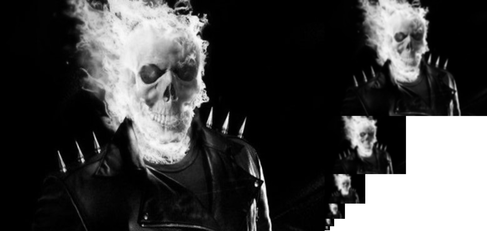
So, we can safely set \(\sigma=2\) for our gaussian filter kernel and get a Gaussian Pyramid as follows

The process has been demonstrated in grayscale, however if the process is repeated for each of the color channels individual, RGB images can be processed like wise. 

Laplacian Pyramid

Once we have the Gaussian Pyramid, deriving the Laplacian Pyramid from it is a piece of cake. The process is as follows:

1. The coarsest scale is the same as that in the Gaussian Pyramid
2. Each subsequently finer level \(I_L(i)\) is obtained by upsampling the next coarser level in the Gaussian Pyramid, \(I_G(i+1)\) to the size of the current level (\(i^{th}\) level) and subtracting it from \(I_G(i)\). The upsampling requires interpolation but MATLAB has a 'imresize' function that does the operation for us, so we're cool for the moment.

The Laplace Pyramid for the above image looks like this

Often the name 'Laplacian' is thought to be a misnomer since nowhere we are taking double derivatives. However, the difference of gaussians is actually an approximation to the laplacian operator upto a scale factor as can be seen below. The argument is simplified using the fact that being Linear Time Invariant operators the order of Derivative and Gaussian Filter can be interchanged. Thus filtering an image with gaussian and then taking derivative is equivalent to filtering the image with the derivative of the gaussian filter. 

\begin{align}
\text{Let } g(x,y;\sigma) &=\frac{1}{2\pi \sigma^2}e^{-\frac{x^2+y^2}{2\sigma^2}} \\
\nabla^2 g(x,y;\sigma) &= \frac{\partial^2 g}{\partial x^2}+ \frac{\partial^2 g}{\partial y^2}\\
 &= \left(\frac{x^2+y^2}{\sigma^2}-1\right)\frac{1}{\sigma^2}g(x,y;\sigma)\\
\frac{\partial g}{\partial \sigma} &= \left(\frac{x^2+y^2}{\sigma^2}-1\right)\frac{1}{\sigma}g(x,y;\sigma)\\
\implies \nabla^2 g(x,y;\sigma) &=\frac{1}{\sigma}\frac{\partial g}{\partial \sigma}\\
&\approx \frac{1}{\sigma}\frac{g(x,y;\sigma+\Delta \sigma)-g(x,y;\sigma)}{\Delta \sigma}
\end{align}

The Laplacian Pyramid representation is useful because it is possible to reconstruct the image from it using the following algorithm:

       for (i=levels-1;i>=1;i++) {

          temp=upsample \(I_L(i+1)\) to the size of \(I_L(i)\);

                        \(I_L(i)\)=\(I_L(i)\)+temp;

       }

       return \(I_L(i)\);

Finally, we are ready to understand Image Blending.

Image Blending

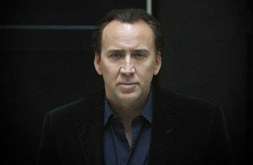
The first task is to manually align the two images to be blended. We need to ensure that the two images are of the same size and somewhat compatible otherwise the blend is going to look like a forced mixture rather than a work of art. I have chosen the following two images

Next, we need to create a mask or a matrix which is the same size as these two images and is filled with 0's wherever we want to see more of The Rider and 1's wherever we want to see Johnny Blaze. My mask looks like this

Now, for the interesting part!! If we simply club the two images together the color contrast and misalignment of edges and details would work against the aesthetic appeal of the image. To tackle this problem the 'blending' must take place across different scales to achieve a smooth transition between the two halves. Also as we move inwards towards the junction from either left or right direction, the pixel values should borrow more and more properties from the other side to create the 'blend'.

Our approach is to first construct the Laplacian Pyramid of the blended image from the Laplacian Pyramids of the two component images and the Gaussian Pyramid of the mask. The blended image is then reconstructed from the blended pyramid. We have already been through the latter step. So, let us see how to obtain the blended pyramid.

This is done as follows. Each of the layers of the blended pyramid \(I_{Lb}(i;x,y)\) is a obtained as a linear combination of the the two component pyramids \(I_{Lc1}(i;x,y)\) and \(I_{Lc2}(i;x,y)\) where the coefficients are functions of the values in the corresponding level in the Gaussian Pyramid of the mask \(I_{Gm}(i;x,y)\)

\begin{align}
I_{Lb}(i;x,y)=(1-I_{Gm}(i;x,y)) \times I_{Lc1}(i;x,y) + (I_{Gm}(i;x,y)) \times I_{Lc2}(i;x,y)
\end{align}

That seals our deal with the devil. Behold the beauty of our creation. Notice how the color of the Blaze's face and hair has developed an orangish glow to match that of The Rider's fire. More is the smoothing in the mask greater is the blending. However, the smoothing can not be overdone as it would lead to too much spill over across the junction. 

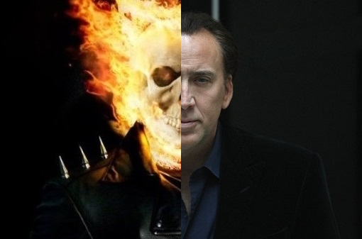
Two two halves clubbed together. Note the stark contrast at the junction

Two halves blended together. The gaussian pyramid of the mask was constructed using kernel with standard deviation 2

Two halves blended together. The gaussian pyramid of the mask was constructed using kernel with standard deviation 10

You know what!! There is a reason why The Ghost Rider has a rating of 5.2 on IMDB. It was the poor quality of Graphics used in the film. You just need to compare the original poster of the movie with the masterpiece that we have created to see this through x)

ALL MATLAB CODE CAN BE FOUND HERE

Its only a matter of "Perspective"

We all have our own different way of looking at situations in life. Not only are there inter class variations, i.e differences between separate individuals, but there are significant intra class variations also, i.e the opinion of an individual is a function of time. The question is why?

Though I don't expect you to ask me for my opinion, I will give it anyway. Well my best guess is that these variations are manifestations of changes and differences in our position in the larger social structure that we are a part of and the unique path that each of has chosen that lands us all in different positions in the frame of reference of the situation. This mapping from our individualism to our take on any problem is highly nonlinear which renders us incapable of seeing others' viewpoint, unless of course, we are really good regressors. By the way you are a geek if you got that joke :p

The situation is quite similar when we are dealing with images. Today we are going to look at how to see an image from different perspectives. Consider a situation where your friend took a photograph standing at a point facing north-north-east. But you really want to see what the image looks like when you are facing north. Theoretically any two planes in 3-D space are related by a transformation known as a Homography and you can always do such a transformation. But before we dig our teeth into Homography we need to understand Perspective projection which is the most widely used model for representing image formation in a camera. Take a look at the schematic below:

Perspective projection in camera

The above image tells you two things- first that I probably copied it from some Spanish website and secondly it tell us how we can model image capture of a 3-D point onto the image plane. Consider \(F_c\) as the origin of the world's 3-D coordinate system. The plane \(z=f\)  is the image plane on which the 3-D scene is projected. For example a point P with world coordinates \((X,Y,Z)\) is projected to a point \((u,v,f)\) in the image plane. The relation between \(P\) and its projection on the image plane is staring us in the face

\[
\frac{X}{Z}=\frac{u}{f}\;\;\;\;
\frac{Y}{Z}=\frac{v}{f}
\]

Clearly the vectors \((X,Y,Z)\) and \((u,v,f)\) are equal up to a scale factor. Which brings us to the notion of homogeneous coordinates. This encapsulates the idea that as long as we know the ray passing through a point we can always choose our image plane by fixing \(f\), the focal length. Coordinate \(P\) is represented in homogeneous coordinates by

\[
\tilde{P}=(\frac{X}{Z},\frac{Y}{Z},1)
\]

Also note that the homogeneous representation of P and that of its projection are equal. You must have guessed by now that there is some relation between the pixel indices and the homogeneous coordinates. While this relation depends on the application, we shall look at one possible interpretation. In images, pixels are usually indexed from the top-left corner. So first we need to normalize the indices so that they lie between \([-1, 1]\) along the larger dimension. This is done by a simple operation

\[
S=max(Height, Width) \\
u=\frac{2i-Width}{S} \; \; \; \;
v=\frac{2j-Height}{S} \\
\tilde{p}=(u,v,1)
\]  

If at all it is required to change the image plane (which is equivalent to changing the scale), as in the case of Automatic Panorama Stitching, then we multiply the homogeneous coordinates by  a projection matrix

\[
\tilde{p}_0=\begin{bmatrix} f & 0 & 0 \\ 0 & f & 0\\0 & 0 & 1 \end{bmatrix} \times \left[ \begin{array}{c} u \\ v \\1 \end{array} \right] = K\tilde{p}
\]

For our purpose \(K\) is simply a $3\times 3$ Identity matrix.

Now coming back to our objective, i.e looking at a photograph taken by your friend in the North-North-East direction from the "perspective" of a person facing North, let us assume that the image taken by your friend is this

Image taken by your friend facing NNE

In order to understand the problem let us look at our coordinate system in a little detail

I hope this schematic does freak you out, because I spent a hell lot of my time making it :p. But its not all that complicated to understand. So first we need to understand that we are dealing with 3 coordinate systems here:
1) Global frame of reference, denoted by \([x,y,z]\), in which we know the positions of the two cameras
2) Frame of reference of your friends camera, denoted by \([x_1,y_1,z_1]\), in which we know the positions of each of the pixels on the image plane. A point in the "Global" frame of reference could be mapped to this coordinate system using a linear mapping

\[
\left[\begin{array}{c} x_1 \\ y_2 \\z_3 \end{array} \right] =R_1 \times \left[\begin{array}{c} x \\ y \\z \end{array} \right]
\]

where \(R_1\) is a \(3\times 3\) rotation matrix. You can use any of the representations of rotation matrix but in my code I've used the axis-angle representation in which one needs to specify the axis of rotation \(\hat{n}\) and the angle of rotation \(\theta\). Since any rotation matrix is orthogonal, the inverse mapping is as simple as

\[
\left[\begin{array}{c} x \\ y \\z \end{array} \right] =R_1^T \times \left[\begin{array}{c} x_1 \\ y_2 \\z_3 \end{array} \right]
\]

In our case the rotation matrix \(R_1\) is parameterized by
\[
\theta=\frac{3 \pi}{2} \; \; \; \; \hat{n}=[0,1,0]
\]
3) Frame of reference in which we want to visualize the scene captured by our friend. This is marked by \([x_2,y_2,z_2]\). Rotation matrix \(R_2\) for this coordinate system is similarly parameterized by
\[
\theta=\frac{11 \pi}{8} \; \; \; \; \hat{n}=[0,1,0]
\]

So now that we have gotten that out of the way, the question that we must answer is what is the transformation from our friends image plane to ours? The answer is now pretty simple and is known as a Homography
\begin{align}
\tilde{p_N}&=\alpha K_N R_N R_{NNE}^TK_{NNE}^{-1}\tilde{p}_{NNE} \\
&= \alpha H\tilde{p}_{NNE}
\end{align}

Note that the factor \(\alpha\) is there simply to account for the fact that two homogenous coordinates are equal as long as they differ only by a scale factor.

That was as far as the theory goes. Now, there are two ways of practically doing this transformation - forward warping and inverse warping with one of them emerging as a clear winner.

Forward Warping
In this procedure each pixel is first normalized as discussed earlier and then transformed using the Homography matrix. But when we convert the homogeneous coordinates back to the pixel coordinates, there is no guarantee that we get integral values. On the contrary, most of the points would lie some between the integer valued pixels.

Source: Marco Zuliani's lectures on Image Warping at UCSB

One way to deal with this problem is to round off the coordinates to integer values. This as you can imagine would result in multiple intensity values from the original image being mapped to the same pixel in the new image while leaving some holes in the new image where no intensity value got mapped. Look at the following example to see what I mean

Forward warped image blatantly showing the problem of holes

Another possible solution could be to assign each integral coordinate the pixel intensity which is nearest to it. Though I haven't tried it out, according to literature, while the holes would fill up, the image starts displaying effects of aliasing. This brings us to our other alternative Inverse Warping.

Inverse Warping
In this method we do an inverse mapping to project each point in the target grid on the source grid, i.e the image plane of our friend. Then the pixel intensities are chosen based on a bilinear interpolation from the neighbouring pixels. Sounds complicated, right! Yes it is........No, I am kidding....its simple. Just look at the image below and go through the description. Then kick yourself if you don't get it right the first time :p

When inverse mapping land you in a non-integer coordinate point

Say, the inverse homography landed you at a non-integer coordinate point $(p,q)$ in your friends image. The intuition is that the pixel intensity at this point should be a linear combination of the intensities at the corners with closer corners getting a higher weight in proportion to the closeness to this point. Thus the intensity at  $(p,q)$ is given by
\begin{align}
I=(1-\Delta x)(1-\Delta y) I(x,y) + (1-\Delta x)(\Delta y) I(x,y+1) \\
+ (\Delta x)(\Delta y) I(x+1,y+1) + (\Delta x)(1-\Delta y) I(x+1,y)
\end{align}

Now behold the beauty of this beast

Brilliance of Inverse Warping

Isn't this a beauty!! You've got to admit this is kinda wicked :D....no ugly distortions....no holes....I feel like an artist looking at his creating. Nah...Lets scrap the sentimental talk.

Not only can you do such simple transformations, but more complicated transformations as well for example feast your eyes on the following results

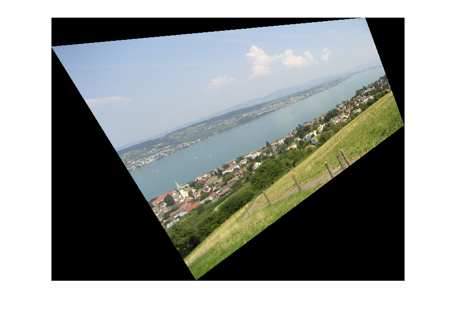
A more interesting Homography using Forward Warping

The more interesting Homography using Inverse Warping

I would urge my readers to understand that while we are defining the Homography manually here , most applications such as Panorama Stitching requires the estimation of Homography using some matching keypoints in different images such as those given by SIFT descriptors. This knowledge renders much of the process discussed above unnecessary but of  course Homography estimation brings other challenges with itself. However, I feel that this exercise that we went through is particularly informative and useful to get a sense of what's going on.

Code shall be uploaded soon, it needs some serious cleaning and commenting to be useful to anybody :p

Seeing through Chaos: Noise Filtering

Mind is a powerful thing. It is both the cause of chaos in our lives and the source of our redemption from it.

 This chaos which religion describes as an "Act of God", is known to Geeks as "Noise". Obviously Rockstars are oblivious to the fact that they are actually pleading for "Chaos" when they ask their audience to "Make some Noise \m/".

Today let us attempt to see through this veil of randomness and uncover the Signals hidden behind. By the way, a very prosperous and a happy new year to all my readers, if that makes you feel any better :p. 

Noise removal using Wiener Filter

A noisy image is an eyesore, yuck! So do we fold our hands and stare at it helplessly. No, we protest....vehemently. We oppose it, suppress it and humiliate it....yeah!! You can't disagree once you've seen this:

Left: Original Image                                                    Right: Noisy Image 

The noise that you are seeing here is called 'Additive White Gaussian Noise'. It is additive because the noise signal (yeah! noise is also a signal, a pathetic one at that but a signal indeed) is algebraically added to the pixel intensities. It is 'Gaussian' because the magnitude of noise at any particular pixel is Gaussian distributed random variable. It is 'white' because just as white light is composed of all possible wavelengths of light, white noise contains all possible frequency components i.e. its Power Spectral Density (PSD) is flat. But what the hell is 'Power Spectral Density' right? Let us dig deeper here because wiener filter stands on the pedestal of PSD and its estimation for the signals in question is absolutely essential.

Power Spectral Density

The idea of PSD resonates with that of Fourier Transforms, in fact by definition for continuous time signals:

\begin{align}PSD(\omega)=E[|F(\omega)|^2] \end{align}

where \(F(\omega)\) is the Fourier Transform of signal \(f(t)\) and \(E[.]\) denotes the expected value. Basically as the name suggests it is a measure of the power contributed by the different frequency components to the original signal. The task of finding the PSD for any deterministic signal such as an image is simple. Because images are discrete signals (at least on computer where the computation takes place), we shall use Discrete Fourier Transform (DFT) instead of the continuous one. For deterministic images, such as the original cameraman image above:

\begin{align}PSD[m,n] = \frac{1}{MN}|F[m,n]|^2 \end{align}

Let me tell you a secret - Continuous-time Fourier Transform (CFT), Discrete-Time Fourier Transform (DTFT) and Discrete Fourier Transform (DFT) used to give me a headache until recently when the concepts began to gel in. So, if you are passing through the same bad weather, may God bless you with one of my future posts :p. Here's a quick hand-wavy recap:

When a continuous time function is sampled, then in frequency domain its transform replicates after intervals of \(\frac{2 \pi}{T}\). Further the transform undergoes both frequency scaling (by a factor of T) and amplitude scaling (by a factor of  1/T) where T is the time period. However for discrete computations in frequency domain in computers we need to sample even the DTFT and because of the periodicity property only the section between \([0, 2 \pi]\) is used. So in this interval for a 1-D signal, for example, the relation between DTFT (\(F(\omega)\)) and DFT \(F[k]\) is given by:

\begin{equation}F[k]=F(\omega)|_{\omega=\frac{2 \pi k}{N}}\end{equation}

As far as the noise is concerned, since we are dealing with AWGN, its PSD is simply the noise variance at all frequencies. What could be simpler than that right?

The Wiener Filter

The idea of Wiener Filter is intuitive. We want to suppress those DFT coefficients where the Signal-to-Noise ratio is small while leaving those coefficients untouched where the Signal-to-Noise ratio is large. Wiener Filter is actually an optimal filter in the sense that it minimizes the mean squared error between the noisy signal and the underlying signal. A rigorous derivation is uploaded here.  But the final result i.e. the filter in frequency domain is give by:

\begin{equation}H(\omega)=\frac{S_u}{S_u+S_\eta}\end{equation}

where \(S_u\) and \(S_\eta\) are the PSD of the original image and noise respectively. This was what the professor who taught me image processing, but who shall remain unnamed here, told me. And I was like: This dude must be crazy! How is it possible to find the PSD of the original image when we are given just the noisy image. But it turns out that a reasonable estimate can be obtained from the noisy image as well. Now I don't know if this is a standard practice but my approach was this:

The trick here is to first perform a Gaussian smoothing operation on the noisy image. This acts as a low pass filter and filters out the high frequency noise components. The PSD of the resulting image would then serve as a not-too-bad estimate of the original image. Of course, now there is a trade-off because Gaussian smoothing also smudges the image. More the smudge, more is the noise that would be filtered out and vice versa. Take your time to appreciate the results below and you can find the entire MATLAB code here.

Noisy image after Gaussian smoothing operation

           Left: Noisy Image                       Right: Wiener Filtered Image

Wiener Filtering using the PSD of original image

There was some gap between my last blog and this one. The reason being I promised you, my readers, that I would tell you how to filter out noise from a signal. I did not expect that I would run into practical issues which we seldom think about while trying to understand the theory. The point is I learnt a lot myself while preparing for this particular blog. Hope you enjoyed it and found it equally informative.

The legacy of Jean Baptiste Joseph Fourier

Vladimir Nabokov, a Russian novelist once said:

"The breaking of a wave cannot explain the whole sea"

I tend to disagree and today I'm gonna try and convince you that Vladimir couldn't be any further from the truth. To prove my point I would like to call the Ghost of Jean Baptiste Joseph Fourier into the witness box.

ME: Tell us Joseph, do you agree with Vladimir?

JOSEPH: Well...I think our friend's remark might explain a lot of philosophical questions as it is indeed true that in order to get the complete picture it is simply not enough to understand a few bits and pieces of it. To be called the master of one's creation, a person has to understand all the pieces of the puzzle and how they fit together.

ME: Did Vladimir pay you for saying all this?

JOSEPH: Oh no, no! I was just getting to the point that while his words have great value in the world of Philosophy, it stands no chance in the ruthless world of mathematics. Through more than 200 years of study, initiated by my work on 'Fourier Series', it has been rigorously proved that periodic signals can be expressed as a sum of very simple oscillating functions, namely sines and cosines (or complex exponential) each oscillating at an integer multiple of the fundamental frequency.

ME: Did you copy that line from Wikipedia or something? Anyways, continue.

JOSEPH: If you have a continuous time periodic function \(f(x)\) (satisfying some criteria for convergence, of course) with period 2L, then it can be written as a linear combination or a weighted sum of complex exponential functions as follows
\begin{equation}
f(x)=\sum_{n=-\infty}^{\infty}A_n e^{\frac{\iota 2 \pi n x}{2 L}} \\
where \: A_n = \frac{1}{2L} \int_{-L}^{L}f(x)e^{\frac{\iota 2 \pi n x}{2 L}} dx
\end{equation}
ME: Dude, you're talking French.

JOSEPH: Let me explain with the help of an example. Consider a square wave with unit amplitude and a period of 2 seconds. A quick calculation shows that the Fourier Series expansion of this particular signal is given by
\begin{equation}
f(x)=\sum_{n=1}^{\infty} \frac{2}{\pi n}(1-(-1)^n) sin({\frac{ \pi n x}{ L}})
\end{equation}
ME: Yeah...right, that would've been a very quick calculation :p

JOSEPH: You can take a look at both my code and calculations if you are inquisitive enough. Click here, c'mon now don't be shy!

ME: Alright I got the calculation but what's the meaning of all this.

JOSEPH: I'm glad you asked that. What the above equation says, is that if you know the Fourier coefficients, not one or two, but all of them then you know the signal completely and it is possible to reconstruct the signal from them.

ME: But doesn't that justify Vladimir's statement then....the need to know all the pieces of the puzzle....all the waves in the sea :-(

JOSEPH: Not quite :-). Look at the image below where I've taken the sum of the first few terms in the Fourier expansion. I want you to notice that as the number of terms are increased from 10 to 1000 the quality of the reconstructed signal increases greatly and I can bet on the Eiffel Tower that with just a 1000 coefficients you won't be able to distinguish between a true square wave and a reconstructed one with just your naked eye.

ME: Ok...that kinda makes sense. But why is there an overshoot at the point of discontinuity.

JOSEPH: Ahem....I was.....umm....I was trying to avoid this discussion but now that you have asked, it is because of something called the Gibbs phenomenon. It happens whenever you try to take the partial sum of the Fourier series of a piecewise continuous signal. Don't give me that look....it is not my mistake. I bet if the computers you've made had infinite precision and were capable of adding the infinitely many terms in the series then the results would have been perfect.

ME: Alright Joseph, but you know there is a fundamental problem. Many signals in nature are continuous time but we must use digital computers to process them, so what use is all that you've told us.

JOSEPH: I think I must leave now for the gates of heavens are closing. Some bloke called Einstein is going to deliver a lecture on some hypothetical theory of Relativity. But two of my proponents Prof. Alan. V. Oppenhiem (MIT) and Prof. Ronald. W. Schafer (Hewlett Packard) have written a book on Digital Signal Processing which addresses this issue in great details.

ME: Your Honor, my witness has given enough evidence to suggest that, breaking a signal into its component harmonics often gives valuable insight about the signal itself. Even today, in applications like speech recognition and image compression Fourier Coefficients are used to encode the signals. With this note I rest my case.

In my next blog, I will skip a few steps i.e. the subtle relationship between Fourier Series, Discrete Time Fourier Transform and Discrete Fourier Transform and really get into how breaking a signal into component frequencies finds use in noise filtering. I know I promised to do it in this blog itself but some foundation had to be established. Anyways its my blog and I can change my mind whenever I want :p.

Despite all my efforts to be accurate and technically correct, some mistakes might have crept in. Please feel free to point them out in the comments bellow.

The Philosophy and Science of Signals

Our lives as humans are meaningful because we are constantly interacting with our environment. Ladies and gentlemen we are in dynamic equilibrium with the states of the universe which is sustained only by an influx of information from sensory receptors in our body and our capability to rationalize and respond to this stimulus, sending fresh waves of change rippling through time and space. Scientists have studied these waves of information and change over a few centuries trying to understand and manipulate them. Today we all know these waves of change as “Signals”.

The range of studies conducted on Signals are diverse. Steve Wozniak might be interested in variations of voltage and current with time in the Apple motherboard. Steve Jobs on the other hand would probably be more interested in the ‘time-series’ of stock prices of Apple which are yet another type of discrete-time signals. Siri is obsessed with speech signals i.e. the variation of voice amplitude over time. And I am a fan of motion pictures which are variations in pixel intensities over both time and space (since any snapshot at a given time is an image which can be looked at as variation of pixel values over the span of the display screen). 

Interestingly computers can be taught to analyse signals to extract the required information and this is a common theme that runs along all problems studied under the broad domain of Signal Processing. Just like food processing is important to convert raw food into edible form before it can be cooked, Signal Processing is important to reduce complex signals into rudimentary forms which can be consumed by the limited intelligence and rationale that computers possess. 

For example, say a satellite picture of region around the Pantheon in Rome (a top view) is to be used to automatically register the total built up area i.e. the floor area occupied by all the buildings in the image. A possible way to tackle the problem is to write a computer program to detect the edges in the image and assuming that the edges corresponding to the view of the rooftops of the building would form closed loops, the program could simply count the number of pixels completely enclosed by loops. In this problem the method of detecting an edge is studied under Image Processing which forms a part of the algorithm for the task of inferring the built up area which is of interest to a researcher in Computer Vision.

Smoothing the image while preserving edge information using Perona-Malik Diffusion

Edge Detection applied to the diffused image using Canny Edge Detection Algorithm

This doesn't look simple and it isn't :p (I love this tongue-sticking-out smiley). Edge detection is done in 2 steps because if Canny edge detection is used on the original image directly then a lot of unnecessary edges are captured which may make the task even more difficult. Thus the image is first smoothed out using a sophisticated algorithm known as Anisotropic Diffusion developed by and named after Pietro Perona (Professor and Computer Vision Researcher at Caltech) and Jitendra Malik (Professor and Computer Vision Researcher at UC, Berkeley). Further as can be seen from the edges detected, our assumption about the loops being closed doesn't hold in many places and it is the job of a Computer Vision researcher to either work his way around this problem or improve the algorithm for edge detection or both.

This example clearly elucidates the dependence of Computer Vision on Signal Processing, especially Image Processing. There are other challenges involved too. For instance, the process of image acquisition by the satellite and transmission to the base station on the ground adds some noise which are random variations that corrupt the original signal. Noise is the manifestation of the imperfect world we live in. Noise removal is a pre-processing step in many applications including the one in question. All is well and good while there is sunshine and a clear sky, but what if clouds come in between the Pantheon and the satellite? That would be hilarious wouldn't it :p ?

Fortunately, Signal Processing deals with techniques that can filter out these unwanted additions to our good old signal like noise and cloud cover (yes! you can look through the clouds) and hence these methods are aptly called Filtering techniques. They come in varying degrees of complexity and applicability.

If you are as excited as I am, then watch out for my next post where we will explore a fundamental concept in Signal Processing and see how it can help us in noise removal in simple 1-D signals.

Guys and girls, please feel free to leave behind a comment. Older people, who don't think they fit into the category of guys and girls, need not refrain from doing so either :-) .

Code for Anisotropic Diffusion and Canny Edge Detection in Matlab

Initializing()

To begin with, the title of this post makes sense if you have ever written a computer program :p.
This is my first ever blog post so do try and be kind, but that's definitely not a prerequisite for following my blog.

The reasons why I have started this blog are as follows:
1. I am about to enter the final semester of my undergraduate education in Electrical Engineering and I am waiting for the results of my PhD applications. So, I have some free time that I would like to fill up with an interlude.
2. I am really fascinated by certain inter-disciplinary topics such as Computer Vision, Machine Learning and Image Processing (Computer Science and Electrical Engineering being the disciplines in question) and I wanted to share my thoughts with the world as I explore.

This blog might be useful for people who stumbled upon the idea that computers might someday take over our world (thanks to Hollywood which seems to be thoroughly excited by the idea and prospects of endless profits the idea might fetch at the Box Office) and would like to know exactly how human researchers have been facilitating it.

But on a more serious note, this century might see a remarkable change in how computers interpret this world of humans and make logical inferences from it. It might be worthwhile to participate if not lead the revolution. So, together let us embark on a journey into how Artificial Intelligence plays a role in our lives today and fathom how this might change in a couple of decades.