There is always more to art than what meets the eye. Throughout ages there have been mysteries and puzzles lurking behind those lines and patterns on canvas and artists go to great lengths to master and execute those techniques which have ushered in a new era of photorealism. Digital arts have taken it to a whole new level by enabling artists to do more with just a click of button. But that 'click' of the button encapsulates a series of mathematical operations that are oblivious to even the most profound artists of our time. Therein lies our opportunity for revelation :p. So just let your brain neurons fire away happily 'cause
Creativity is intelligence having fun-Albert Einstein
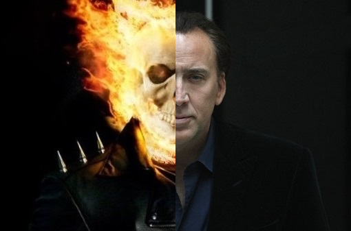
You might be wondering as to what the poster of Ghost Rider is doing on a blog titled 'A Human In a Machine's Word', The Rider being neither a human nor a machine. Well it is here because it is an excellent example of a digital art form known as Image Blending in which two layers of different images - that of Johnny Blaze and the Ghost Rider in this instance, are seamlessly and aesthetically blended together. Such images are often created using commercial software like Adobe Photoshop. Today we shall try and understand what goes at the backend while creating such effects and then create our own masterpiece using Computer Vision techniques.
But first we need to understand the concept of Gaussian and Laplacian Image Pyramids.
Gaussian Pyramid
An image pyramid is a multi-scale representation of an image that allows the processing of an image at different resolutions. It is basically a collection of images derived from the original image using some mathematical operations. However, all pyramid representations have two properties in common:
- The subsequent images are smaller than the current image, usually by a factor of 2. Thus, when the images are stacked together in the order of decreasing size, the stack resembles a pyramid and hence the name 'Image Pyramid'
- The base of the pyramid captures the high frequency characteristics of the image, i.e, finer details (such as edges and texture) whereas the subsequent layers capture the low frequency characteristic or the coarser features in the image (such as object silhouettes and appearance)
In the case of gaussian pyramid, represented as \(I_G(n)\) to denote the \(n^{th}\) level of the gaussian pyramid of image \(I(x,y)\), each subsequent layer is a gaussian smoothed and sampled version of the previous image. This deserves a deeper look.
Whenever a signal is sampled in the time domain, its Fourier transform replicates. For example, if \(X(\Omega)\) is the Fourier Transform of a 1D signal \(x[n]\), then the Fourier Transform of a sampled but zero-padded version of the signal \(x_p[n]\) formed by selecting every \(N^{th}\) value from the original signal while suppressing the remaining values to 0 is given by \(X_p(\Omega)\) as shown below. The actually subsampled signal \(x_d[n]\) is formed by compressing the zero-padded signal. Clearly if a signal is compressed by a factor of \(\frac{1}{N}\), then its Fourier Transform is expanded by a factor of \(N\).
Notice that the fourier transform of the original signal and its final sampled version is similar except for magnitude and frequency scaling factors. This is an ideal situation and the sampled image looks like the original image just smaller in size. However, if \(\Omega_M\) is large, so that the replicas begin to overlap then the fourier transform of the final sampled version gets distorted and is no longer similar to that of the original signal. This phenomenon is known as Aliasing. To avoid this situation, i.e, to prevent overlap between the replicas, it is essential for the following condition to hold
\begin{align}
\Omega_M < \frac{2\pi}{N}-\Omega_M
\implies \Omega_M < \frac{\pi}{N}
\end{align}
This is the great Nyquist Theorem, sampling rate \(\frac{1}{N}\) must be at least twice the cut-off frequency to avoid aliasing (replace \(\Omega_M\) by \(2 \pi f_{cutoff}\) ). Unfortunately, real world signals more often than not fall prey to Aliasing. To deal with this situation the frequencies that would otherwise overlap with the replicas are chopped off prior to sampling by using a low-pass filter. Of course, there would be some high frequency losses, i.e some loss of details, but still we are much better off than the aliased versions. It turns out that filtering by a gaussian kernel in spatial domain is equivalent to passing the image through a low pass filter, provided the standard deviation of the kernel is chosen to be large enough. The reason is that Fourier Transform of a Gaussian is also a Gaussian
\begin{align}
\frac{1}{\sqrt{2\pi}\sigma}e^{-\frac{x^2}{2\sigma^2}} \leftrightarrow e^{-2\pi^2 \sigma^2 u^2}
\end{align}
The latter is a Gaussian with a standard deviation of \(\sigma_0=\frac{1}{2\pi \sigma}\). Now for a Gaussian 99% of its area is accounted for by the interval \([-3\sigma_0, 3\sigma_0]\). Hence its cut-off frequency can be safely assumed to be \(3\sigma_0\). Using the Nyquist Theorem with \(N=2\) gives us
\[\sigma > \frac{6}{\pi}\]
\begin{align}
\Omega_M < \frac{2\pi}{N}-\Omega_M
\implies \Omega_M < \frac{\pi}{N}
\end{align}
This is the great Nyquist Theorem, sampling rate \(\frac{1}{N}\) must be at least twice the cut-off frequency to avoid aliasing (replace \(\Omega_M\) by \(2 \pi f_{cutoff}\) ). Unfortunately, real world signals more often than not fall prey to Aliasing. To deal with this situation the frequencies that would otherwise overlap with the replicas are chopped off prior to sampling by using a low-pass filter. Of course, there would be some high frequency losses, i.e some loss of details, but still we are much better off than the aliased versions. It turns out that filtering by a gaussian kernel in spatial domain is equivalent to passing the image through a low pass filter, provided the standard deviation of the kernel is chosen to be large enough. The reason is that Fourier Transform of a Gaussian is also a Gaussian
\begin{align}
\frac{1}{\sqrt{2\pi}\sigma}e^{-\frac{x^2}{2\sigma^2}} \leftrightarrow e^{-2\pi^2 \sigma^2 u^2}
\end{align}
The latter is a Gaussian with a standard deviation of \(\sigma_0=\frac{1}{2\pi \sigma}\). Now for a Gaussian 99% of its area is accounted for by the interval \([-3\sigma_0, 3\sigma_0]\). Hence its cut-off frequency can be safely assumed to be \(3\sigma_0\). Using the Nyquist Theorem with \(N=2\) gives us
\[\sigma > \frac{6}{\pi}\]
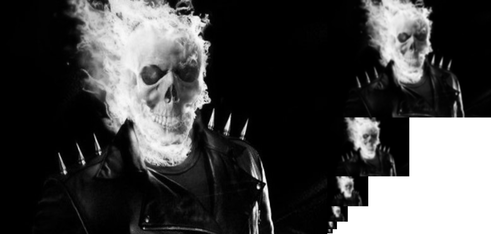
So, we can safely set \(\sigma=2\) for our gaussian filter kernel and get a Gaussian Pyramid as follows
The process has been demonstrated in grayscale, however if the process is repeated for each of the color channels individual, RGB images can be processed like wise.
\begin{align}
\text{Let } g(x,y;\sigma) &=\frac{1}{2\pi \sigma^2}e^{-\frac{x^2+y^2}{2\sigma^2}} \\
\nabla^2 g(x,y;\sigma) &= \frac{\partial^2 g}{\partial x^2}+ \frac{\partial^2 g}{\partial y^2}\\
&= \left(\frac{x^2+y^2}{\sigma^2}-1\right)\frac{1}{\sigma^2}g(x,y;\sigma)\\
\frac{\partial g}{\partial \sigma} &= \left(\frac{x^2+y^2}{\sigma^2}-1\right)\frac{1}{\sigma}g(x,y;\sigma)\\
\implies \nabla^2 g(x,y;\sigma) &=\frac{1}{\sigma}\frac{\partial g}{\partial \sigma}\\
&\approx \frac{1}{\sigma}\frac{g(x,y;\sigma+\Delta \sigma)-g(x,y;\sigma)}{\Delta \sigma}
\end{align}
The process has been demonstrated in grayscale, however if the process is repeated for each of the color channels individual, RGB images can be processed like wise.
Laplacian Pyramid
Once we have the Gaussian Pyramid, deriving the Laplacian Pyramid from it is a piece of cake. The process is as follows:- The coarsest scale is the same as that in the Gaussian Pyramid
- Each subsequently finer level \(I_L(i)\) is obtained by upsampling the next coarser level in the Gaussian Pyramid, \(I_G(i+1)\) to the size of the current level (\(i^{th}\) level) and subtracting it from \(I_G(i)\). The upsampling requires interpolation but MATLAB has a 'imresize' function that does the operation for us, so we're cool for the moment.
The Laplace Pyramid for the above image looks like this
Often the name 'Laplacian' is thought to be a misnomer since nowhere we are taking double derivatives. However, the difference of gaussians is actually an approximation to the laplacian operator upto a scale factor as can be seen below. The argument is simplified using the fact that being Linear Time Invariant operators the order of Derivative and Gaussian Filter can be interchanged. Thus filtering an image with gaussian and then taking derivative is equivalent to filtering the image with the derivative of the gaussian filter.
\begin{align}
\text{Let } g(x,y;\sigma) &=\frac{1}{2\pi \sigma^2}e^{-\frac{x^2+y^2}{2\sigma^2}} \\
\nabla^2 g(x,y;\sigma) &= \frac{\partial^2 g}{\partial x^2}+ \frac{\partial^2 g}{\partial y^2}\\
&= \left(\frac{x^2+y^2}{\sigma^2}-1\right)\frac{1}{\sigma^2}g(x,y;\sigma)\\
\frac{\partial g}{\partial \sigma} &= \left(\frac{x^2+y^2}{\sigma^2}-1\right)\frac{1}{\sigma}g(x,y;\sigma)\\
\implies \nabla^2 g(x,y;\sigma) &=\frac{1}{\sigma}\frac{\partial g}{\partial \sigma}\\
&\approx \frac{1}{\sigma}\frac{g(x,y;\sigma+\Delta \sigma)-g(x,y;\sigma)}{\Delta \sigma}
\end{align}
The Laplacian Pyramid representation is useful because it is possible to reconstruct the image from it using the following algorithm:
for (i=levels-1;i>=1;i++) {
temp=upsample \(I_L(i+1)\) to the size of \(I_L(i)\);
\(I_L(i)\)=\(I_L(i)\)+temp;
}
return \(I_L(i)\);
Finally, we are ready to understand Image Blending.
Image Blending
The first task is to manually align the two images to be blended. We need to ensure that the two images are of the same size and somewhat compatible otherwise the blend is going to look like a forced mixture rather than a work of art. I have chosen the following two images

Next, we need to create a mask or a matrix which is the same size as these two images and is filled with 0's wherever we want to see more of The Rider and 1's wherever we want to see Johnny Blaze. My mask looks like this
Now, for the interesting part!! If we simply club the two images together the color contrast and misalignment of edges and details would work against the aesthetic appeal of the image. To tackle this problem the 'blending' must take place across different scales to achieve a smooth transition between the two halves. Also as we move inwards towards the junction from either left or right direction, the pixel values should borrow more and more properties from the other side to create the 'blend'.
Our approach is to first construct the Laplacian Pyramid of the blended image from the Laplacian Pyramids of the two component images and the Gaussian Pyramid of the mask. The blended image is then reconstructed from the blended pyramid. We have already been through the latter step. So, let us see how to obtain the blended pyramid.
This is done as follows. Each of the layers of the blended pyramid \(I_{Lb}(i;x,y)\) is a obtained as a linear combination of the the two component pyramids \(I_{Lc1}(i;x,y)\) and \(I_{Lc2}(i;x,y)\) where the coefficients are functions of the values in the corresponding level in the Gaussian Pyramid of the mask \(I_{Gm}(i;x,y)\)
I_{Lb}(i;x,y)=(1-I_{Gm}(i;x,y)) \times I_{Lc1}(i;x,y) + (I_{Gm}(i;x,y)) \times I_{Lc2}(i;x,y)
\end{align}
That seals our deal with the devil. Behold the beauty of our creation. Notice how the color of the Blaze's face and hair has developed an orangish glow to match that of The Rider's fire. More is the smoothing in the mask greater is the blending. However, the smoothing can not be overdone as it would lead to too much spill over across the junction.
 |
| Two two halves clubbed together. Note the stark contrast at the junction |
 |
| Two halves blended together. The gaussian pyramid of the mask was constructed using kernel with standard deviation 2 |
 |
| Two halves blended together. The gaussian pyramid of the mask was constructed using kernel with standard deviation 10 |
You know what!! There is a reason why The Ghost Rider has a rating of 5.2 on IMDB. It was the poor quality of Graphics used in the film. You just need to compare the original poster of the movie with the masterpiece that we have created to see this through x)


