We all have our own different way of looking at situations in life. Not only are there inter class variations, i.e differences between separate individuals, but there are significant intra class variations also, i.e the opinion of an individual is a function of time. The question is why?
Though I don't expect you to ask me for my opinion, I will give it anyway. Well my best guess is that these variations are manifestations of changes and differences in our position in the larger social structure that we are a part of and the unique path that each of has chosen that lands us all in different positions in the frame of reference of the situation. This mapping from our individualism to our take on any problem is highly nonlinear which renders us incapable of seeing others' viewpoint, unless of course, we are really good regressors. By the way you are a geek if you got that joke :p
The situation is quite similar when we are dealing with images. Today we are going to look at how to see an image from different perspectives. Consider a situation where your friend took a photograph standing at a point facing north-north-east. But you really want to see what the image looks like when you are facing north. Theoretically any two planes in 3-D space are related by a transformation known as a Homography and you can always do such a transformation. But before we dig our teeth into Homography we need to understand Perspective projection which is the most widely used model for representing image formation in a camera. Take a look at the schematic below:
The above image tells you two things- first that I probably copied it from some Spanish website and secondly it tell us how we can model image capture of a 3-D point onto the image plane. Consider \(F_c\) as the origin of the world's 3-D coordinate system. The plane \(z=f\) is the image plane on which the 3-D scene is projected. For example a point P with world coordinates \((X,Y,Z)\) is projected to a point \((u,v,f)\) in the image plane. The relation between \(P\) and its projection on the image plane is staring us in the face
\[
\frac{X}{Z}=\frac{u}{f}\;\;\;\;
\frac{Y}{Z}=\frac{v}{f}
\]
Clearly the vectors \((X,Y,Z)\) and \((u,v,f)\) are equal up to a scale factor. Which brings us to the notion of homogeneous coordinates. This encapsulates the idea that as long as we know the ray passing through a point we can always choose our image plane by fixing \(f\), the focal length. Coordinate \(P\) is represented in homogeneous coordinates by
\[
\tilde{P}=(\frac{X}{Z},\frac{Y}{Z},1)
\]
Also note that the homogeneous representation of P and that of its projection are equal. You must have guessed by now that there is some relation between the pixel indices and the homogeneous coordinates. While this relation depends on the application, we shall look at one possible interpretation. In images, pixels are usually indexed from the top-left corner. So first we need to normalize the indices so that they lie between \([-1, 1]\) along the larger dimension. This is done by a simple operation
\[
S=max(Height, Width) \\
u=\frac{2i-Width}{S} \; \; \; \;
v=\frac{2j-Height}{S} \\
\tilde{p}=(u,v,1)
\]
If at all it is required to change the image plane (which is equivalent to changing the scale), as in the case of Automatic Panorama Stitching, then we multiply the homogeneous coordinates by a projection matrix
\[
\tilde{p}_0=\begin{bmatrix} f & 0 & 0 \\ 0 & f & 0\\0 & 0 & 1 \end{bmatrix} \times \left[ \begin{array}{c} u \\ v \\1 \end{array} \right] = K\tilde{p}
\]
For our purpose \(K\) is simply a $3\times 3$ Identity matrix.
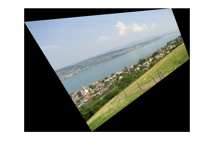
Now coming back to our objective, i.e looking at a photograph taken by your friend in the North-North-East direction from the "perspective" of a person facing North, let us assume that the image taken by your friend is this
In order to understand the problem let us look at our coordinate system in a little detail

I hope this schematic does freak you out, because I spent a hell lot of my time making it :p. But its not all that complicated to understand. So first we need to understand that we are dealing with 3 coordinate systems here:
1) Global frame of reference, denoted by \([x,y,z]\), in which we know the positions of the two cameras
2) Frame of reference of your friends camera, denoted by \([x_1,y_1,z_1]\), in which we know the positions of each of the pixels on the image plane. A point in the "Global" frame of reference could be mapped to this coordinate system using a linear mapping
\[
\left[\begin{array}{c} x_1 \\ y_2 \\z_3 \end{array} \right] =R_1 \times \left[\begin{array}{c} x \\ y \\z \end{array} \right]
\]
where \(R_1\) is a \(3\times 3\) rotation matrix. You can use any of the representations of rotation matrix but in my code I've used the axis-angle representation in which one needs to specify the axis of rotation \(\hat{n}\) and the angle of rotation \(\theta\). Since any rotation matrix is orthogonal, the inverse mapping is as simple as
\[
\left[\begin{array}{c} x \\ y \\z \end{array} \right] =R_1^T \times \left[\begin{array}{c} x_1 \\ y_2 \\z_3 \end{array} \right]
\]
In our case the rotation matrix \(R_1\) is parameterized by
\[
\theta=\frac{3 \pi}{2} \; \; \; \; \hat{n}=[0,1,0]
\]
3) Frame of reference in which we want to visualize the scene captured by our friend. This is marked by \([x_2,y_2,z_2]\). Rotation matrix \(R_2\) for this coordinate system is similarly parameterized by
\[
\theta=\frac{11 \pi}{8} \; \; \; \; \hat{n}=[0,1,0]
\]
So now that we have gotten that out of the way, the question that we must answer is what is the transformation from our friends image plane to ours? The answer is now pretty simple and is known as a Homography
\begin{align}
\tilde{p_N}&=\alpha K_N R_N R_{NNE}^TK_{NNE}^{-1}\tilde{p}_{NNE} \\
&= \alpha H\tilde{p}_{NNE}
\end{align}
Note that the factor \(\alpha\) is there simply to account for the fact that two homogenous coordinates are equal as long as they differ only by a scale factor.
That was as far as the theory goes. Now, there are two ways of practically doing this transformation - forward warping and inverse warping with one of them emerging as a clear winner.
Forward Warping
In this procedure each pixel is first normalized as discussed earlier and then transformed using the Homography matrix. But when we convert the homogeneous coordinates back to the pixel coordinates, there is no guarantee that we get integral values. On the contrary, most of the points would lie some between the integer valued pixels.
One way to deal with this problem is to round off the coordinates to integer values. This as you can imagine would result in multiple intensity values from the original image being mapped to the same pixel in the new image while leaving some holes in the new image where no intensity value got mapped. Look at the following example to see what I mean
Another possible solution could be to assign each integral coordinate the pixel intensity which is nearest to it. Though I haven't tried it out, according to literature, while the holes would fill up, the image starts displaying effects of aliasing. This brings us to our other alternative Inverse Warping.
Inverse Warping
In this method we do an inverse mapping to project each point in the target grid on the source grid, i.e the image plane of our friend. Then the pixel intensities are chosen based on a bilinear interpolation from the neighbouring pixels. Sounds complicated, right! Yes it is........No, I am kidding....its simple. Just look at the image below and go through the description. Then kick yourself if you don't get it right the first time :p
Say, the inverse homography landed you at a non-integer coordinate point $(p,q)$ in your friends image. The intuition is that the pixel intensity at this point should be a linear combination of the intensities at the corners with closer corners getting a higher weight in proportion to the closeness to this point. Thus the intensity at $(p,q)$ is given by
\begin{align}
I=(1-\Delta x)(1-\Delta y) I(x,y) + (1-\Delta x)(\Delta y) I(x,y+1) \\
+ (\Delta x)(\Delta y) I(x+1,y+1) + (\Delta x)(1-\Delta y) I(x+1,y)
\end{align}
Now behold the beauty of this beast
Isn't this a beauty!! You've got to admit this is kinda wicked :D....no ugly distortions....no holes....I feel like an artist looking at his creating. Nah...Lets scrap the sentimental talk.
Not only can you do such simple transformations, but more complicated transformations as well for example feast your eyes on the following results
I would urge my readers to understand that while we are defining the Homography manually here , most applications such as Panorama Stitching requires the estimation of Homography using some matching keypoints in different images such as those given by SIFT descriptors. This knowledge renders much of the process discussed above unnecessary but of course Homography estimation brings other challenges with itself. However, I feel that this exercise that we went through is particularly informative and useful to get a sense of what's going on.
Code shall be uploaded soon, it needs some serious cleaning and commenting to be useful to anybody :p
Though I don't expect you to ask me for my opinion, I will give it anyway. Well my best guess is that these variations are manifestations of changes and differences in our position in the larger social structure that we are a part of and the unique path that each of has chosen that lands us all in different positions in the frame of reference of the situation. This mapping from our individualism to our take on any problem is highly nonlinear which renders us incapable of seeing others' viewpoint, unless of course, we are really good regressors. By the way you are a geek if you got that joke :p
The situation is quite similar when we are dealing with images. Today we are going to look at how to see an image from different perspectives. Consider a situation where your friend took a photograph standing at a point facing north-north-east. But you really want to see what the image looks like when you are facing north. Theoretically any two planes in 3-D space are related by a transformation known as a Homography and you can always do such a transformation. But before we dig our teeth into Homography we need to understand Perspective projection which is the most widely used model for representing image formation in a camera. Take a look at the schematic below:
 |
| Perspective projection in camera |
The above image tells you two things- first that I probably copied it from some Spanish website and secondly it tell us how we can model image capture of a 3-D point onto the image plane. Consider \(F_c\) as the origin of the world's 3-D coordinate system. The plane \(z=f\) is the image plane on which the 3-D scene is projected. For example a point P with world coordinates \((X,Y,Z)\) is projected to a point \((u,v,f)\) in the image plane. The relation between \(P\) and its projection on the image plane is staring us in the face
\[
\frac{X}{Z}=\frac{u}{f}\;\;\;\;
\frac{Y}{Z}=\frac{v}{f}
\]
Clearly the vectors \((X,Y,Z)\) and \((u,v,f)\) are equal up to a scale factor. Which brings us to the notion of homogeneous coordinates. This encapsulates the idea that as long as we know the ray passing through a point we can always choose our image plane by fixing \(f\), the focal length. Coordinate \(P\) is represented in homogeneous coordinates by
\[
\tilde{P}=(\frac{X}{Z},\frac{Y}{Z},1)
\]
Also note that the homogeneous representation of P and that of its projection are equal. You must have guessed by now that there is some relation between the pixel indices and the homogeneous coordinates. While this relation depends on the application, we shall look at one possible interpretation. In images, pixels are usually indexed from the top-left corner. So first we need to normalize the indices so that they lie between \([-1, 1]\) along the larger dimension. This is done by a simple operation
\[
S=max(Height, Width) \\
u=\frac{2i-Width}{S} \; \; \; \;
v=\frac{2j-Height}{S} \\
\tilde{p}=(u,v,1)
\]
If at all it is required to change the image plane (which is equivalent to changing the scale), as in the case of Automatic Panorama Stitching, then we multiply the homogeneous coordinates by a projection matrix
\[
\tilde{p}_0=\begin{bmatrix} f & 0 & 0 \\ 0 & f & 0\\0 & 0 & 1 \end{bmatrix} \times \left[ \begin{array}{c} u \\ v \\1 \end{array} \right] = K\tilde{p}
\]
For our purpose \(K\) is simply a $3\times 3$ Identity matrix.
Now coming back to our objective, i.e looking at a photograph taken by your friend in the North-North-East direction from the "perspective" of a person facing North, let us assume that the image taken by your friend is this
 |
| Image taken by your friend facing NNE |
In order to understand the problem let us look at our coordinate system in a little detail
I hope this schematic does freak you out, because I spent a hell lot of my time making it :p. But its not all that complicated to understand. So first we need to understand that we are dealing with 3 coordinate systems here:
1) Global frame of reference, denoted by \([x,y,z]\), in which we know the positions of the two cameras
2) Frame of reference of your friends camera, denoted by \([x_1,y_1,z_1]\), in which we know the positions of each of the pixels on the image plane. A point in the "Global" frame of reference could be mapped to this coordinate system using a linear mapping
\[
\left[\begin{array}{c} x_1 \\ y_2 \\z_3 \end{array} \right] =R_1 \times \left[\begin{array}{c} x \\ y \\z \end{array} \right]
\]
where \(R_1\) is a \(3\times 3\) rotation matrix. You can use any of the representations of rotation matrix but in my code I've used the axis-angle representation in which one needs to specify the axis of rotation \(\hat{n}\) and the angle of rotation \(\theta\). Since any rotation matrix is orthogonal, the inverse mapping is as simple as
\[
\left[\begin{array}{c} x \\ y \\z \end{array} \right] =R_1^T \times \left[\begin{array}{c} x_1 \\ y_2 \\z_3 \end{array} \right]
\]
In our case the rotation matrix \(R_1\) is parameterized by
\[
\theta=\frac{3 \pi}{2} \; \; \; \; \hat{n}=[0,1,0]
\]
3) Frame of reference in which we want to visualize the scene captured by our friend. This is marked by \([x_2,y_2,z_2]\). Rotation matrix \(R_2\) for this coordinate system is similarly parameterized by
\[
\theta=\frac{11 \pi}{8} \; \; \; \; \hat{n}=[0,1,0]
\]
So now that we have gotten that out of the way, the question that we must answer is what is the transformation from our friends image plane to ours? The answer is now pretty simple and is known as a Homography
\begin{align}
\tilde{p_N}&=\alpha K_N R_N R_{NNE}^TK_{NNE}^{-1}\tilde{p}_{NNE} \\
&= \alpha H\tilde{p}_{NNE}
\end{align}
Note that the factor \(\alpha\) is there simply to account for the fact that two homogenous coordinates are equal as long as they differ only by a scale factor.
That was as far as the theory goes. Now, there are two ways of practically doing this transformation - forward warping and inverse warping with one of them emerging as a clear winner.
Forward Warping
In this procedure each pixel is first normalized as discussed earlier and then transformed using the Homography matrix. But when we convert the homogeneous coordinates back to the pixel coordinates, there is no guarantee that we get integral values. On the contrary, most of the points would lie some between the integer valued pixels.
 |
| Source: Marco Zuliani's lectures on Image Warping at UCSB |
 |
| Forward warped image blatantly showing the problem of holes |
Inverse Warping
In this method we do an inverse mapping to project each point in the target grid on the source grid, i.e the image plane of our friend. Then the pixel intensities are chosen based on a bilinear interpolation from the neighbouring pixels. Sounds complicated, right! Yes it is........No, I am kidding....its simple. Just look at the image below and go through the description. Then kick yourself if you don't get it right the first time :p
 |
| When inverse mapping land you in a non-integer coordinate point |
\begin{align}
I=(1-\Delta x)(1-\Delta y) I(x,y) + (1-\Delta x)(\Delta y) I(x,y+1) \\
+ (\Delta x)(\Delta y) I(x+1,y+1) + (\Delta x)(1-\Delta y) I(x+1,y)
\end{align}
Now behold the beauty of this beast
 |
| Brilliance of Inverse Warping |
Not only can you do such simple transformations, but more complicated transformations as well for example feast your eyes on the following results
 |
| A more interesting Homography using Forward Warping |
 |
| The more interesting Homography using Inverse Warping |
Code shall be uploaded soon, it needs some serious cleaning and commenting to be useful to anybody :p